DeepSeek V4.1 Flash is built around a specific systems problem: an agent repeatedly reads a growing history, generates a smaller amount of new text, pauses for tools, and returns later. Optimising only the arithmetic inside attention leaves substantial costs in prompt processing, cache capacity and moving stored state back to the accelerator.
The design tackles those costs together. Causal Encoder–Decoder (CED) reduces how much of the network most prompt tokens traverse. Compressed Sparse Attention 2 (CSA2) shares stored representations and sparse selections across layers. FP4 cache storage reduces bytes per entry. SWA Bounded Replay reconstructs short-range state when retaining it would be more expensive.
This is a technical reading of DeepSeek-AI’s 51-page report, Pushing the Limits of KV Cache Compression, checked on 11 September 2026 against the released configuration and reference implementation. Section and page references below identify the underlying mechanisms. Calculations and proposed tests are AIEngine’s analysis; performance figures are DeepSeek’s reported results. For availability and pricing, see the separate V4.1 Flash release analysis.
Start with three different kinds of state
An attention cache holds representations of earlier tokens so the model can use them without recomputing the entire history. In this architecture, the global branch and the local sliding-window branch have different storage and reuse patterns.
| State | Purpose | Scaling and lifetime |
|---|---|---|
| Global main KV and indexer K | Retrieve information across the causal history | Grows with context; useful for persistent prefix reuse |
| Layer-local SWA KV | Preserve detailed recent-token interactions | Bounded window per layer; short-lived serving state |
| Engram parameters | Supply learned conditional memory by token-based lookup | Model parameters, independent of a particular conversation’s cache |
In the report’s introduction and inference section, HBM is the accelerator’s high-bandwidth memory, while SSD and host DRAM provide additional storage tiers. A cache can be small in one tier yet expensive to transfer or reconstruct in another.
This distinction prevents a common misreading of the headline: 890 bytes per token describes global KV state, not all inference memory. Model weights, Engram tables, local windows, activations, temporary workspaces, allocation overhead and concurrency still need resources.
The actual 40-layer topology
The language backbone has 40 layers with hidden width 5,120. The bottom 20 form a causal encoder and the top 20 a decoder. Both are causal: the encoder is not a bidirectional document reader that sees future tokens. Each block contains a mixture-of-experts feed-forward layer; the first two attention layers use only SWA, and the remaining 38 add CSA2 global attention.
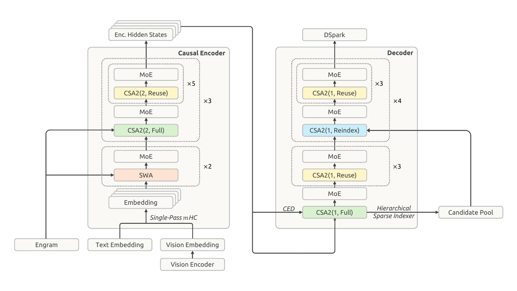
Figure source: section 2.1, page 7. On a narrow screen, scroll the diagram horizontally to inspect the labels.
The released inference configuration makes the schedule unusually concrete. Using zero-based layer numbers:
| Layers | Global compression | CSA2 assignment |
|---|---|---|
| 0–1 | None | SWA only |
| 2–19 | Two tokens per global entry | Three groups: one Full, then five Reuse |
| 20–23 | One token per global entry | One Full, then three Reuse |
| 24–39 | One token per global entry | Four groups: one Reindex, then three Reuse |
Global KV producers are layers 2, 8, 14 and 20. Index-producing layers are 2, 8, 14, 20, 24, 28, 32 and 36. The mode assignment is static, although the selected positions depend on the query. “Full” means the complete CSA2 production-and-selection path; it does not turn the layer into dense attention over every historical token.
Every MoE block has one shared expert and 384 routed experts, with six routed experts selected per token. The report distinguishes 552B backbone parameters from 196B Engram parameters, and reports about 8B activated during prefill versus 16B during decode. Those active counts describe computation through the backbone; they should not be used as a model-weight storage estimate.
CED: build decoder memory without running the whole decoder
In a conventional decoder stack, each layer derives its historical keys and values from that layer’s own hidden states. Building all those caches requires taking the prompt through every layer.
CED changes the source of decoder global KV. In section 2.2, equation 1, decoder global entries and compression weights are projected from the final encoder hidden state. With H20 denoting the output of the first 20 layers, the structural relation is:
C_l = H20 W_KV,l
Z_l = H20 W_Z,l
Here C represents the global KV entries and Z their compression weights. Projection weights are layer-dependent in the CED formulation; the actual CSA2 schedule further shares the resulting global state. A decoder layer still computes its own query from its current representation. Sharing the historical memory does not make the decoder’s attention output identical across layers.
Most prompt positions can therefore finish their expensive processing after the encoder. The remaining complication is local attention: decoder SWA keys and values still depend on each decoder layer’s own hidden state. The serving system reconstructs a bounded suffix to initialise that local state before generation.
Using L layers, N prompt tokens and window W, the report gives the approximate layer-token work:
Conventional prefill:        O(N L)
CED with bounded replay:     O(N L/2 + W L/2)
For N much larger than W:    approximately O(N L/2)
This explains the input/output asymmetry. During generation, a new token traverses both halves; the decoder has not disappeared. The expression also is not a complete latency model: attention, projections, routing, communication, cache hits and scheduling affect wall-clock time. The benefit must be measured separately for long cold prompts and short additions to cached sessions.
CSA2: reuse memory and reuse selection independently
CSA2 combines local SWA with sparse access to global entries. A lightweight indexer chooses global positions, while the main attention query attends to those selected entries together with the local window. The design separates three decisions: who creates memory, who selects positions, and who reads the selected memory.
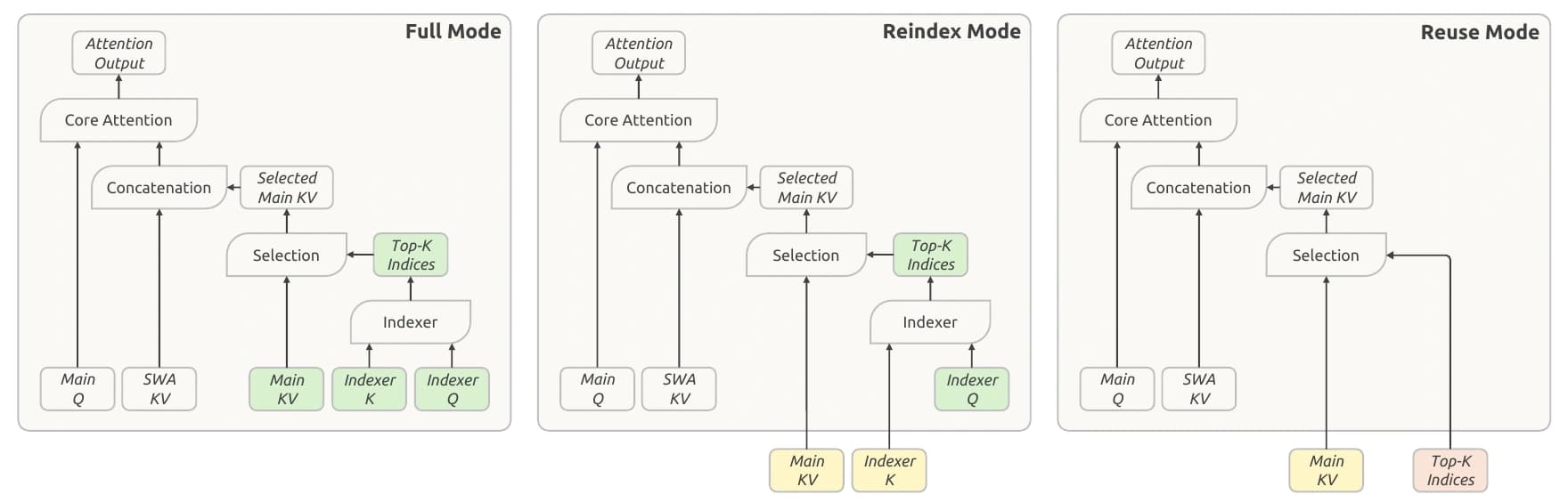
The three modes in section 2.3.1 have different responsibilities:
- Full: creates main KV, derives indexer K, computes indexer Q and selects a fresh Top-K set.
- Reindex: shares an earlier Full layer’s main KV and indexer K, but computes a new indexer query and a new selection.
- Reuse: shares main KV and the latest compatible selection, skipping a fresh indexing pass.
- All modes: compute their own main query, layer-local SWA KV and new attention output.
Cache reuse saves storage. Index reuse saves selection work. Reindex exists because forcing every layer to use one selection would remove the ability to revisit different evidence as representations evolve. Conversely, selecting different evidence need not require another complete stored copy of the history.
CSA2 also simplifies sequence compression. Unlike V4’s overlapping compressor, it groups non-overlapping source positions and removes the compressor’s absolute positional embedding. Indexer K is projected from the main KV representation, rather than produced by an independent compression path from hidden states. V4.1 uses CSA2 throughout the global branch, replacing V4’s CSA/HCA mixture.
The decoder’s compression ratio is one, so its global entries are not reduced along the sequence dimension. It still saves memory through layer sharing and precision. Compression along the entry, sequence and layer dimensions should be counted separately; multiplying headline ratios without checking their overlap can count the same saving twice.
Hierarchical indexing bounds later searches, not every search
The model selects up to 512 global entries per query. An indexer can still be expensive if it scores a million candidate positions before selecting those entries. Sharing selections reduces the number of indexers, but does not reduce the search space of the indexers that remain.
The hierarchical sparse indexer, section 2.3.2, addresses that remaining cost in the decoder:
- The first Full layer scores the entire causally visible global history.
- It chooses its own Top-512 entries for attention.
- It also scores blocks by their maximum position score and retains up to 2,048 blocks of eight positions.
- Those blocks produce a pool of at most 16,384 candidate positions.
- Later Reindex layers select their own Top-512 entries from that pool; Reuse layers inherit the latest selection.
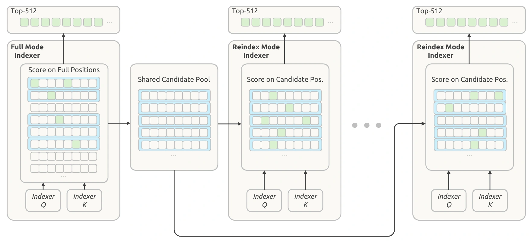
The pool is query-specific and larger than the final attention set. It is neither one fixed shortlist for the entire conversation nor 16,384 entries all passed into core attention.
For context length N and fixed pool P, an illustrative count of positions scored by the decoder’s five indexers changes from roughly 5N to N + 4P. With N = 1,000,000 and P = 16,384, that is 1,065,536 rather than 5,000,000 positions. This is our simplified selection-work comparison, excluding block selection, kernel overhead and encoder indexing; it is not a measured speedup.
The initial full-range scan remains linear in context length. The report’s nearly flat decode-FLOP curve must therefore not be rewritten as constant-time inference. Figure 2 reports precision-weighted arithmetic, with context growing from 4K to 1M increasing the model’s decode FLOPs by about one-quarter. Arithmetic weighting and user-observed latency are different measurements.
Reconstructing the 890-byte cache budget
The reported global KV footprint can be understood from the topology and storage formats. Section 2.4.4 specifies an E2M1 main cache with one E4M3 scale per 16 channels. The reference implementation distinguishes that from the indexer’s 32-channel groups and E8M0 scales.
For the configured 512-channel main KV latent and 128-channel indexer key, the packed storage calculation is:
Main KV:   512 × 4/8 + 512/16 × 1 = 288 bytes
Indexer K: 128 × 4/8 + 128/32 × 1 =  68 bytes
One global entry, including scales: 356 bytes

Encoder: 3 cache producers × N/2 entries = 1.5 N
Decoder: 1 cache producer  × N   entries = 1.0 N

Global state: 2.5 N × 356 = 890 N bytes
This is an analytical reconstruction of the reported packed cache budget, not an allocator measurement from the reference runner. At exactly one million tokens it gives 890 MB in decimal units, or about 849 MiB, for global KV. The factor of 2.5 arises from three compressed encoder caches plus one uncompressed decoder cache. The decoder does not keep twenty separate global histories.
The implementation uses quantisation-aware training for these representations. The main cache is quantised after rotary position encoding and dequantised before attention. Its format resembles NVFP4 but omits the second-level global scale. The report argues that the cache’s normalised dynamic range does not require it. Local SWA KV remains FP8 because it is more sensitive to quantisation.
This is a cache-storage decision, not a claim that every operation or every model weight uses four-bit arithmetic. A deployment must account for padding, scale layout, tensor-parallel replication, temporary tensors and the number of live requests before converting 890 MB into an admission limit.
Bounded replay is deliberately approximate
SWA uses a window of 128 tokens, but dependencies accumulate through layers. Exact reconstruction of L layers’ local state can require replaying roughly L × W tokens. Merely remembering the final 128 input tokens is not mathematically equivalent to having retained all the intermediate hidden states that generated their caches.
DeepSeek makes a deliberate approximation: replay only the last W tokens, truncating local attention at the replay segment’s start. Section 3.2.2, page 20 distinguishes two paths:
| Replay path | Trigger | Treatment of state |
|---|---|---|
| Encoder replay | Global prefix hits, but encoder SWA state is missing | Rebuild local state over the cached suffix; reuse cached global KV without overwriting it |
| Decoder replay | Prefill must initialise decoder local state | Send only the last window’s encoder outputs through the decoder; use that local state for decoding |
The uncached suffix subsequently produces both new global and local state. Because it depends on the approximately reconstructed boundary, its state can vary with the cache-hit position. The report explicitly says these paths are not mathematically identical to full recomputation, while reporting negligible quality impact in its tests. Decoder replay is also simulated during post-training.
This is where the persistent-cache saving comes from. In V4, retained local states occupied nearly half of the persistent cache under the described workload. V4.1 removes them from that long-lived store and further compresses the retained global state by roughly fourfold, giving the reported approximately eightfold persistent reduction.
SWA state is not absent everywhere. The report describes a short-lived distributed host-memory pool for encoder SWA, using 10% of each machine’s host DRAM, with minute-scale retention. Global cache storage has a much longer lifetime in the described deployment. Those are implementation details from the paper, not a retention guarantee for every external provider.
Single-Pass mHC removes a memory dependency
Manifold-constrained hyper-connections maintain multiple residual streams. V4.1 uses four. In the original formulation, coefficients derived from the current residual state determine how that same state is mixed into the next block. Computing the coefficients requires a reduction, so the mixed input must wait and the residual is read again.
In section 2.4.1, Single-Pass mHC shifts the input-mixing coefficient by one block:
Original:    X_(l+1) = B_l X_l + C_l F_l(A_l X_l)
Single-pass: X_(l+1) = B_l X_l + C_l F_l(A_(l-1) X_l)
A mixes residual streams into the block input, B mixes the residual path, and C distributes the block output. Using the previous block’s A removes the immediate dependency on the current coefficient calculation. The Mega-mHC deployment kernel can combine residual update, input mixing, coefficient prediction, pre-normalisation and FP8 conversion in one pass.
The report reduces activation reads plus writes from (4n + 4)d to (2n + 2)d. For n = 4, that is 20d to 10d: a halving of this operation’s activation traffic, not of the model’s total traffic. The mathematical shift enables the fusion; naming a kernel alone would not explain the saving.
Engram and DSpark solve different problems
Engram supplies learned conditional memory. The report’s section 2.4.2 allocates 196B parameters across two modules at zero-based layers 1 and 14. They use 2-, 3- and 4-grams with eight hash heads per order, followed by context-aware integration. Deterministic token-based addressing allows embeddings to be prefetched from host memory while computation proceeds.
These are learned embedding tables, not retrieved web documents or a conversation log. Their footprint belongs in the model’s parameter and placement budget, while the KV cache belongs to the session. During RL rollouts, the report places Engram tables on GPUs to relieve host-memory pressure, illustrating that placement is workload-dependent.
DSpark accelerates generation through speculative decoding. Three draft Transformer blocks produce base logits for five positions in parallel; a lightweight Markov head models dependencies between draft tokens. A confidence head estimates acceptance, and a scheduler combines expected prefix survival with profiled engine throughput to choose how much draft to verify under the current load.
The verifier still determines which draft tokens survive. Five proposed positions do not imply five accepted tokens or a universal fivefold speedup. DSpark is introduced after backbone pretraining with the backbone frozen, then remains aligned during post-training without its objective’s gradients flowing into the backbone.
The minimal inference README is explicit about scope: its model code contains the DSpark forward path, but generation is plain autoregressive sampling. Running that reference is not a reproduction of the production speculative scheduler.
Vision is integrated before language-model pretraining
The image pathway is a separately trained DeepSeek-ViT, a 3 × 3 pixel-unshuffle operation, and a two-layer MLP projector into the language backbone. Section 2.1.1 describes 2D rotary positions, RMSNorm and SwiGLU in the vision encoder. The configuration specifies 32 vision layers, width 1,024, 16 attention heads and 14-pixel patches.
Pixel unshuffle rearranges each spatial neighbourhood into channels, reducing visual token count by nine before projection. As a shape calculation, a 1,344 × 1,344 image divided into 14-pixel patches yields a 96 × 96 grid. Threefold reduction along each axis leaves 32 × 32, or 1,024 visual positions. This explains the configured maximum; actual preprocessing and API billing should be checked in the vision documentation.
Images and text can route differently through the MoE. Separate expert-bias corrections balance the modalities independently, while the original router scores weight the selected expert outputs. Balancing only their combined load could conceal imbalance within one modality.
The pretraining setup, section 4.2, reports 45T tokens, a 7:1 text-only-to-multimodal token mixture, sparse attention trained at 64K from the start, and extension to 1M context at 34T tokens. The vision encoder is initially frozen during joint language-model training and unfrozen at learning-rate decay. “Native multimodal” therefore does not mean every component was trained from random initialisation in one uninterrupted joint stage.
Training and serving complete the design
The optimiser follows parameter structure: Muon for major matrices, head-wise treatment for query and key weights, AdamW for normalisation and other non-matrix parameters, and momentum followed by Sinkhorn balancing for large embeddings and the prediction head. The latter avoids Adam’s second-moment buffer on enormous tables. Sharing attention state across pipeline stages also requires managing forward transfers, backward gradient accumulation and release of shared buffers; it is not just a forward-pass pointer alias.
The serving system in section 3.2 separates vision encoding, prefill and decode so they can scale independently. Fused kernels reduce the overhead of the many conceptual components. The report counts 15 kernels for prefill and 11 for decode in a CSA2 Reuse layer. That count describes the documented implementation, rather than a guarantee for every open-source runtime.
Post-training retains SFT, RL and on-policy distillation. DeepSeek attributes the substantive changes to task and environment synthesis, data quality and rollout scale. Its effort control conditions training on a scalar b from 1 to 100, with group-relative comparisons made within the same prompt and effort level. An effort-dependent token penalty decreases exponentially as b rises, letting higher effort spend more tokens.
The report maps public low, high and max presets to 50, 75 and 100. The current API guide exposes those named tiers. Intermediate research values and public request parameters are separate interfaces. The paper’s results at maximum effort should not be assumed to describe the default high tier’s cost or accuracy.
What the evidence establishes—and what to test next
The report describes a coherent memory hierarchy and reports strong model-level results. It does not establish that each individual mechanism causes a particular benchmark gain. Architecture, training data, reinforcement learning and inference configuration changed together. Our assessment is that attributing the entire gain to CSA2, or to any single component, would require additional controlled ablations.
Section 6 explicitly identifies sparse-selection errors and approximate state reconstruction as incompletely characterised robustness boundaries. The practical implication is to test the decisions where the system discards alternatives or rebuilds missing state:
| Test | Failure it can expose | Evidence to retain |
|---|---|---|
| Move essential evidence across distant positions and block boundaries | Candidate selection misses relevant context | Accuracy by evidence position and context length |
| Resume the same prefix at different hit boundaries | Bounded replay changes a consequential result | Cache boundary, output and task-level correctness |
| Compare warm SWA hits with replay after eviction | Recovery cost or quality differs from the warm path | Time to first token, cache state and correctness |
| Sweep low, high and max on identical tasks | Effort changes budget without a useful quality gain | Total tokens, latency, success and review time |
| Vary images, aspect ratios and text density | Preprocessing or vision failures | Original image, processed shape and extraction errors |
| Increase concurrency and shorten turns | Cache movement or scheduling dominates arithmetic | Throughput, tail latency and per-tier memory |
These are proposed experiments, not tests AIEngine has already run on the model. Cache-boundary differences should be graded by task correctness as well as numerical differences: stochastic output variation alone is not evidence of a regression. A controlled runtime comparison should hold prompts, sampling, harness and resource limits constant.
For reproduction, pin the checkpoint, configuration, prompt format, runtime and harness. The encoding package and deepseek-recipe cover protocol-aware prompt conversion. Their presence does not supply the production scheduler, persistent-cache service or tool-execution environment. Our broader guide to LLM memory architectures provides context for comparing this design with linear-attention and recurrent-memory approaches.
The most instructive feature of V4.1 Flash is the alignment between what the model computes, what it stores, and what the serving system is willing to reconstruct. CED makes global decoder memory available early; CSA2 reduces duplicated history and repeated search; cache precision reduces each stored representation; replay trades exact retained local state for bounded recomputation. Understanding those separate contracts makes the efficiency claim both more convincing and more testable.
Figures 3, 4 and 5 are reproduced from DeepSeek-AI’s technical report. The model repository supplies an MIT licence; the copyright and permission notice accompanies the locally hosted figures. The analysis uses the report downloaded on 11 September 2026; live documentation may subsequently change.