State
What the model keeps from prior tokens.
Update
How new information edits that state.
Retrieval
How sequence and depth information return.
In 2019, the small public GPT-2 checkpoint had 124 million parameters. In 2026, Kimi K3 arrived with 2.8 trillion total parameters, 104 billion activated for each token, a one-million-token context window and a hybrid architecture built around Kimi Delta Attention and Attention Residuals. Divide 2.8 trillion by 124 million and the result is about 22,580.
That comparison is mathematically correct and architecturally incomplete. It compares total parameters with the smallest GPT-2 release, not active compute with active compute. More importantly, seven years of progress changed the model's memory system: what is stored, how it is updated, what can be forgotten and how information can be retrieved across both sequence length and network depth.
This technical literature expands the complete original X Article by @waterloo_intern into a paper-linked field guide. It follows the same intellectual path—GPT-2, linear attention, fast-weight memory, DeltaNet, gated DeltaNet, Kimi Delta Attention, Kimi K3 and AttnRes—while separating established mechanism, reported result and engineering interpretation.
The 22,580× number needs three denominators
The headline uses the 124M GPT-2 small model because that is the clean decoder-only baseline reproduced in many teaching implementations. OpenAI also released 355M, 774M and 1.5B GPT-2 variants. The GPT-2 technical report describes the full 1.5B model, while OpenAI's release timeline documents the staged 124M checkpoint.
Kimi K3 is a sparse Mixture-of-Experts model. Its technical report gives 2.8T total parameters but 104B activated parameters. A token therefore does not traverse all 2.8T parameters.
| Comparison | Ratio to GPT-2 small | What it means |
|---|---|---|
| Kimi K3 total parameters: 2.8T ÷ 124M | 22,580× | Total learned capacity across shared and routed components |
| Kimi K3 activated parameters: 104B ÷ 124M | About 839× | A closer, still imperfect per-token capacity comparison |
| Kimi K3 total: 2.8T ÷ GPT-2 1.5B | About 1,867× | Comparison with the largest released GPT-2 |
None of these ratios is an inference-cost ratio. Runtime also depends on sequence length, activated experts, arithmetic precision, memory movement, kernel fusion, batch shape, parallelism and serving hardware. That distinction matters when connecting model architecture to the full production AI cost stack.
GPT-2 gives us the clean decoder baseline
GPT-2 is a decoder-only Transformer trained to predict the next token. For an input sequence, it adds learned token embeddings to learned position embeddings, passes the result through a stack of pre-normalised Transformer blocks, applies a final normalisation and projects the last hidden state into vocabulary logits.
A simplified forward path looks like this:
x = token_embedding(token_ids) + position_embedding(positions)

for block in transformer_blocks:
    x = x + causal_self_attention(layer_norm_1(x))
    x = x + mlp(layer_norm_2(x))

logits = language_model_head(final_layer_norm(x))
next_token = sample(logits[:, -1])
The small configuration uses 12 layers, 12 attention heads and a 768-dimensional residual stream. Its conceptual simplicity is useful: each layer alternates a token-mixing operation—causal multi-head self-attention—with a channel-mixing operation—the MLP. Residual connections preserve and accumulate information through depth.
During training, every position can predict its next token in parallel because the future is masked. During generation, only the newest position's logits select the next token. Without caching, each decode step would recompute keys and values for all earlier tokens.
That observation produces the KV cache.
The bottleneck is different in prefill and decode
It helps to split inference into two phases.
Prefill processes the prompt. Standard causal attention forms query, key and value projections for all prompt tokens, then evaluates masked token-to-token interactions. Naively materialising the full attention matrix costs quadratic memory in sequence length.
Decode adds one token at a time. A practical implementation stores the keys and values produced for earlier tokens. The new query reads that history, attends over it and appends one new key and value. Compute per decode step grows with context length, and the cache occupies more memory as the sequence grows.
FlashAttention changed how exact softmax attention executes. Its tiled, IO-aware algorithm avoids materialising the entire attention matrix in high-bandwidth memory and reduces data movement between HBM and on-chip SRAM. It does not change the attention function, and it does not make the historical keys and values vanish during autoregressive decoding.
This distinction resolves a common confusion:
- FlashAttention attacks intermediate-memory traffic for exact attention.
- KV caching avoids recomputing prior key and value projections.
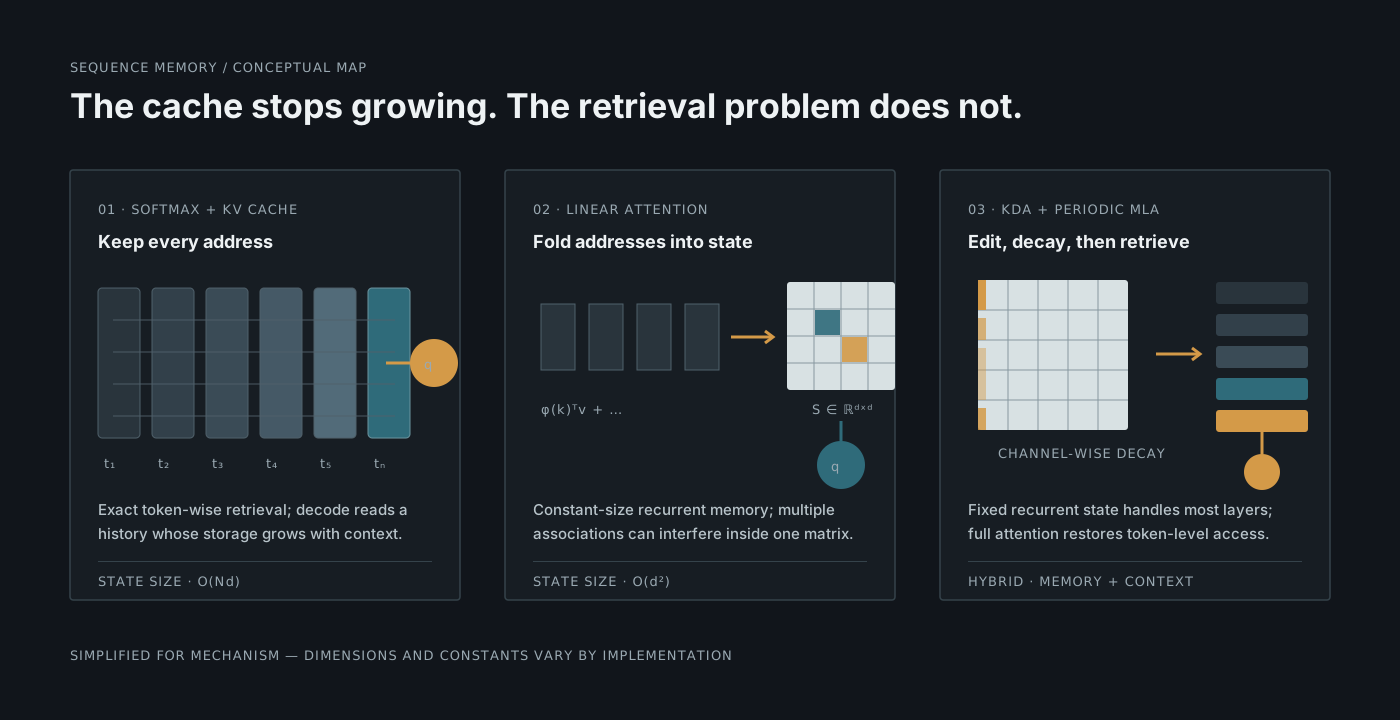
- Linear attention changes the algebra so prior tokens can be folded into a fixed-size state.
Linear attention changes the order of multiplication
Softmax attention computes similarity scores before multiplying by values:
softmax(QKᵀ / √d)V
The softmax couples each query to the complete key set. That makes the expression difficult to reassociate into a fixed recurrent state.
The 2020 paper Transformers are RNNs replaces softmax attention with a kernel feature map. Apply a non-negative transformation φ to queries and keys, then use matrix associativity:
φ(Q)(φ(K)ᵀV)
Instead of storing every key-value pair, the model accumulates a matrix state and a normalisation vector:
q = feature_map(q)              # non-negative query features
k = feature_map(k)              # non-negative key features

state = state + outer(k, v)      # S_t = S_(t-1) + k_t^T v_t
normalizer = normalizer + k

numerator = q @ state
denominator = q @ normalizer
output = numerator / denominator
For recurrent decoding, state size no longer grows with the number of tokens. The model reads a fixed matrix instead of a token-indexed cache. Sequence mixing becomes linear in sequence length, and the relationship to a recurrent neural network becomes explicit.
The saving comes with a semantic price. A KV cache preserves distinct token addresses. A fixed matrix combines associations. The system has compressed “which value belonged to which key” into a finite associative memory.
A fixed matrix eventually enters an overcapacity regime
The fast-weight interpretation makes the limitation easier to see. The Linear Transformers Are Secretly Fast Weight Programmers paper treats the matrix state as a rapidly programmed memory. Each token writes an outer product of its key and value. A later query retrieves a weighted combination from that matrix.
Purely additive memory never removes anything:
state = state + outer(key, value)When keys are sufficiently distinct and capacity is not exceeded, retrieval can work well. As more associations occupy the same finite state, keys overlap and writes interfere. The regime where sequence length is much larger than the feature dimension is precisely where constant-state memory is most attractive—and where capacity pressure is most visible.
The problem is no longer cache growth. It is memory management.
An effective fixed-capacity memory needs answers to four questions:
- What does the current key already retrieve?
- How much should this token change that association?
- Which unrelated content should decay?
- When should the model bypass compressed state and retrieve from full context?
DeltaNet, gated DeltaNet, KDA and hybrid MLA layers answer those questions in stages.
The delta rule makes associative memory editable
A blind additive update writes the whole new value even when much of that value is already stored. The delta rule first reads the memory at the current key, compares that read with the desired value, and writes only the error.
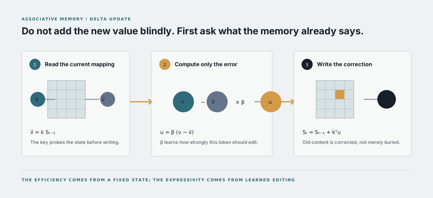
In a compact row-vector convention:
old_value = key @ state
correction = beta * (value - old_value)
state = state + key.transpose(-1, -2) @ correction
output = query @ state
The learned scalar β is a write strength. If the memory already returns the target value, the correction approaches zero. If the stored mapping is wrong, the update removes the conflicting component and writes the replacement.
This is why “fast-weight programmer” is more than a metaphor. The slow network, trained by gradient descent, emits keys, values and update strengths that program a second, rapidly changing matrix during the forward pass.
The delta rule improves targeted editing, but a direct implementation is sequential. Token t needs the state produced at token t−1 before it can calculate its correction. That dependency is unfriendly to accelerators built for large parallel matrix multiplications.
Chunkwise DeltaNet makes the recurrence hardware-usable
The 2024 Parallelizing Linear Transformers with the Delta Rule paper reparameterises the update with products of Householder transition matrices. The key engineering result is a chunkwise algorithm that separates two forms of work:
- Within a chunk: compute masked token-to-token interactions in parallel.
- Across chunks: carry one recurrent matrix state from the previous chunk.
For sequence length L, head dimension d and chunk size C, the paper gives work on the order of O(LCd + Ld²) with O(L/C) sequential steps. The chunk size is therefore a hardware trade-off.
At C = 1, the operation is maximally recurrent and uses fewer arithmetic operations, but tiny kernels underuse the GPU. At C = L, it approaches ordinary quadratic attention. Intermediate chunks—often sizes aligned with tensor-core-friendly tiles—spend extra arithmetic to expose useful parallelism.
The conceptual forward pass is:
for chunk in sequence:
    # Read everything stored before this chunk.
    inter_chunk = q_chunk @ state

    # Compute causal interactions and delta corrections inside the chunk.
    correction = solve_chunk_delta(k_chunk, v_chunk, beta_chunk, state)
    intra_chunk = causal(q_chunk @ k_chunk.transpose(-1, -2)) @ correction

    output_chunk = inter_chunk + intra_chunk
    state = state + k_chunk.transpose(-1, -2) @ correction
The exact implementation is more involved: the paper's memory-efficient representation avoids materialising every intermediate state while preserving the delta updates. The important progression is that the expressive update rule becomes compatible with matrix-multiply hardware.
Gated DeltaNet separates targeted editing from global forgetting
The delta rule can replace the association addressed by the current key. It cannot efficiently clear many stale associations when the subject changes, a document ends or the model needs to reset part of its working memory.
State-space models provide a complementary idea: decay the previous state before adding the new contribution.
state = alpha * state + new_writeWhen α is near one, memory persists. When α is near zero, prior state is rapidly erased. The Gated Delta Networks paper combines this adaptive decay with the delta rule. Its framing is precise: gating provides rapid memory erasure, while the delta update provides targeted modification.
The two controls solve different problems:
| Mechanism | Control | Strength | Limitation on its own |
|---|---|---|---|
| Delta rule | β, write strength | Correct one addressed association | Cannot cheaply reset unrelated memory |
| State decay | α, persistence | Forget broad state after context change | Treats many channels similarly |
| Gated delta rule | α plus β | Global erase and targeted edit | Coarse decay still limits selectivity |
This combination remains chunk-parallelisable because cumulative decay can be represented with products across positions, analogous to a prefix product rather than a prefix sum.
Kimi Delta Attention makes forgetting channel-specific
Gated DeltaNet uses a scalar-like decay control for a state update. Kimi Delta Attention extends the transition to finer-grained, channel-wise decay. Different state dimensions can retain or erase information at different rates.
The Kimi Linear paper describes KDA as an extension of Gated DeltaNet designed to use finite recurrent memory more effectively. It pairs KDA with Multi-head Latent Attention in a layerwise hybrid, rather than claiming compressed state can replace exact retrieval everywhere.
Under the paper's controlled comparisons, the 48B-total, 3B-active Kimi Linear model outperformed its full-MLA baseline across the evaluated settings. The authors report up to 75% lower KV-cache use and up to 6× decoding throughput at one-million-token context. Those are architecture-paper results under specified models, kernels and workloads—not a universal promise for every deployment.
The architectural lesson is broader than the benchmark number. Capacity is added where it has a defined role:
- KDA supplies compact recurrent memory for most sequence mixing.
- Fine-grained decay acts as a learned eviction policy.
- Periodic MLA restores full softmax retrieval from token context.
- Mixture-of-Experts expands channel-processing capacity without activating every parameter.
This is a hybrid memory system, not “linear attention won and softmax disappeared”.
Kimi K3 scales the hybrid, then adds another retrieval axis
Kimi K3 retains the KDA-plus-MLA language backbone and scales it into a 2.8T-total, 104B-active model. The report describes Stable LatentMoE with 896 routed experts; 16 are activated for each token, alongside shared experts. It also adds native vision and a one-million-token context window.
The complete architecture has 23 four-layer macrocycles. In each cycle, three layers use KDA and the fourth uses MLA. The first feed-forward layer is dense; the remaining layers use latent-space MoE. The X Article's architecture reconstruction also highlights gated MLA, MLA query LoRA, output gating and the SiTU expert activation.
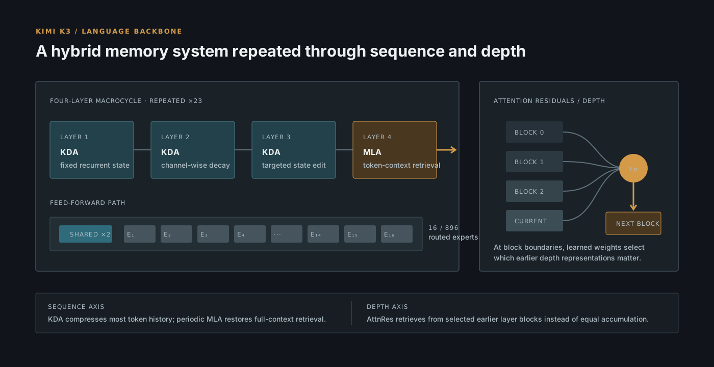
Latent-space MoE is important to the total-versus-active parameter distinction. A router selects a small subset of experts for each token. The model can hold broad specialist capacity without evaluating every expert every time. Stable routing and expert-parallel training then become systems problems as much as modelling problems.
The official Kimi K3 repository publishes weights, technical material and evaluation details. The report attributes its approximately 2.5× overall scaling-efficiency improvement over Kimi K2 to the combination of KDA, AttnRes, Stable LatentMoE and refined training/data recipes. That is a compound result; it should not be assigned to one module in isolation.
AttnRes retrieves across model depth
KDA and MLA deal with information across sequence positions. Attention Residuals address a separate axis: information across layers.
In an ordinary residual stack, a later hidden state contains the accumulated contribution of many earlier blocks. Equal additive accumulation is simple and preserves gradient paths, but it gives the next layer no explicit mechanism for saying “the representation from twelve layers ago is more useful than the immediate predecessor”. As depth grows, useful features can be diluted inside the aggregate residual stream.
AttnRes treats earlier residual blocks as keys and values. A learned query for the current block produces weights over those earlier depth representations, and their weighted combination becomes the input to the next computation. In simplified form:
depth_values = stack(previous_blocks + [partial_block])
depth_keys = normalize(depth_values)

scores = einsum(layer_query, depth_keys)
hidden = einsum(softmax(scores, dim=0), depth_values)
Applying this at every layer would be expensive. Kimi K3 uses blockwise AttnRes at twelve-layer boundaries, creating a lower-frequency retrieval path through depth. The mechanism complements the sequence hierarchy:
- KDA retrieves from compressed recurrent state.
- MLA retrieves from token-level context.
- AttnRes retrieves from earlier depth-level representations.
The model now has selective access along two axes: where information appeared in the sequence, and where a useful representation was created in the network.
What changed at each architectural step
The progression is easiest to remember as a series of repaired failure modes.
| Stage | State | Update rule | Retrieval | Limitation addressed |
|---|---|---|---|---|
| GPT-2 softmax | Token-indexed KV cache | Append K and V | Query all stored keys | Exact retrieval, but growing cache |
| Linear attention | Fixed matrix plus normaliser | Add outer products | Query associative state | Constant state, but interference |
| DeltaNet | Fixed matrix | Read, subtract, gated correction | Query edited state | Targeted replacement |
| Gated DeltaNet | Decaying fixed matrix | Global decay plus delta edit | Query managed state | Context reset and stale memory |
| KDA hybrid | Channel-gated state plus periodic KV | Fine-grained decay and delta edit | KDA state plus MLA context | More selective eviction and exact fallback |
| Kimi K3 | KDA/MLA hierarchy plus depth blocks | Gating, routing, sparse experts | Sequence retrieval plus AttnRes | Capacity across context, experts and depth |
The table also shows why “linear versus quadratic” is too small a framing. Real model design trades retrieval fidelity, state capacity, training parallelism, decode bandwidth, sparse routing, kernel quality and depth-wise information flow.
Engineering implications beyond Kimi K3
Several durable principles fall out of this history.
- Memory size and memory quality are separate. A fixed-size state is valuable only if the update rule preserves useful associations under pressure.
- An eviction policy is part of intelligence. Learned decay, gating and routing determine what the model can stop carrying.
- Exact attention remains a retrieval primitive. Hybrid architectures use it where compressed memory is insufficient.
- Algorithm and kernel must be designed together. A lower-FLOP recurrence can be slower if it cannot occupy the accelerator efficiently.
- Total parameters are not active compute. Sparse experts add capacity, but serving cost follows activation, communication, precision and memory layout.
- Long context is not proof of long-context use. Evaluate retrieval, synthesis and instruction retention at the required lengths. Our enterprise RAG evaluation guide uses the same principle: test the complete evidence path, not the advertised window.
- Every compression layer needs a fallback. KDA has MLA; residual accumulation gains AttnRes; production systems need their own source, human-review and failure-recovery paths.
For engineering teams, the correct question is not “Should we replace attention?” It is: which information must remain exactly addressable, which can be compressed into state, how quickly should that state decay, and what retrieval path repairs inevitable loss?
Source trail and reading order
This article is a synthesis, not a substitute for the papers. A practical reading order is:
- GPT-2: Language Models are Unsupervised Multitask Learners for the decoder-only baseline and scaling context.
- Transformers are RNNs for kernelised attention and recurrent constant-state decoding.
- FlashAttention for exact attention restructured around GPU memory traffic.
- Linear Transformers Are Secretly Fast Weight Programmers for associative-memory capacity and the delta update.
- Parallelizing Linear Transformers with the Delta Rule for chunkwise hardware-efficient DeltaNet.
- Gated Delta Networks for complementary global decay and targeted editing.
- Kimi Linear for fine-grained KDA and the KDA/MLA hybrid.
- Kimi K3: Open Frontier Intelligence and the official repository for the complete 2026 system.
- 22580: From GPT2 to Kimi3, Explained for the original visual worklog that motivated this expanded literature.
The final answer to “is it just scale?” is no—but scale still matters. Kimi K3 combines vastly more learned capacity with a more deliberate memory architecture. Its recurrent state is edited rather than blindly accumulated, decayed rather than allowed to saturate, backed by exact sequence retrieval, expanded through sparse experts and supplemented by attention over depth.
The 22,580× ratio tells us how far parameter count moved. The architecture tells us what that capacity learned to do.